Gas Exchange by Rana and Rameia

Jazmean's Wisconsin Fast Plants Mini Lab

Jazmean Williams

The Effect of Selection Pressures on the Average Leaf Length of Wisconsin Fast Plants

Research Question and Hypothesis

Research Question: Does selection for average leaf length in the Parent Generation influence F1 phenotypes?

Hypothesis: Selection for longer leaf lengths in the P Generation results in a longer leaf average in the F1 Generation due to directional selection.

Results

P Generation Pre-Selection

After planting the seeds and giving them time to grow, the class observed the plants on Day 5 of the experiment. Discussion ensued after looking at the plants and we decid selection process. We then gathered data from the plants. For the P Generation before selection, there were 57 plants. Each student in the class measured the leaf lengths of each plant quad (Figure 1). The measurements of the average leaf lengths of each separate plant aided in deciding which plants were able to stay in the experiment and which ones were cut. After finding what the average leaf lengths were, we graphed the data in the form of a histogram (Figure 2). This was done to see if there was a variation of leaf lengths in this generation and if leaf length was a trait that could be used in the selection process. The histogram showed that there was a variation of leaf lengths in the P Generation and that leaf length could be used in the selection process. The class determined that we were going to selected against small leaf lengths and we chose 12mm as our cut off length. This means that if at least one of the leaves of the plants were 12mm or more, they stayed. If the plant contained no leaves that were at least 12mm, they were cut. The average leaf length of each plant also helped in determining the median and mean leaf length of the P Generation which was 8.5mm and was 8.839mm respectively. We also found the Standard Deviation, SEM, and Confidence Intervals of this generation. Figure 3 shows all of the data collected from the P Generation before selection.

Figure 1



Figure 2

                     

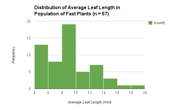
Figure 3

	P Generation
Sample Size (n)	57
Mean	8.839181287 mm
Median	8.5 mm
Standard deviation	3.39196426 mm
SEM	0.4492766416 mm
95% CI Lower Limit	7.940628004 mm
95% CI Upper Limit	9.73773457 mm

P Generation After Selection

After the P Generation underwent the selection process, only 8 plants remained. We calculated the mean and median of the survivor generation which were 13.88 mm and 13.75 mm respectively (Figure 4).  We also calculated the average leaf lengths of the plants and made a histogram of the data (Figure 5). The histogram provided us with a visual representation to see if the leaf lengths were 12mm and above and we selected correctly. To reaffirm that we really did the selection process correctly, we found the Standard Deviation and SEM which helped us find the Upper and Lower Confidence Intervals of the P Generation Survivors. We then compared the intervals with the P Generation Confidence Intervals. Confidence Intervals gives us the parameters of a population. They provide a range of values that, with a certain degree of confidence (in this case, 95%), tell us where the “true” population values fall. If the Confidence Intervals of the P Generation and the P Generation Survivors overlap, we know that they both have a chance of having a plant with the same leaf length. We do not want this since we are selecting against leaf lengths shorter than 12mm. The overlap between the two intervals would also tell us that we did our selection process wrong. Luckily, the two confidence intervals did not overlap (Figure 6). Knowing this allowed us to continue with our experiment. We cross pollinated the plants on Days 12 to 16 of the experiment. After drying the seed pods, we counted 54 seeds in total and replanted them.

Figure 4

	P Generation - Survivors
Sample Size (n)	8
Mean	13.88 mm
Median	13.75 mm
Standard deviation	1.26 mm
SEM	0.45 mm
95% CI Lower Limit	12.98 mm
95% CI Upper Limit	14.78 mm

Figure 5

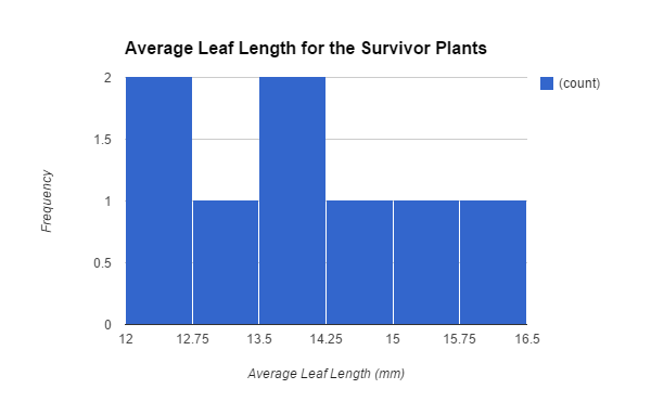
Figure 6

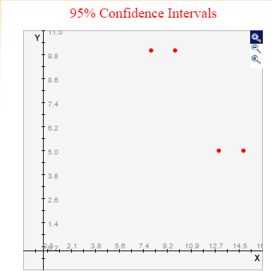
(Top dots are P Generation and bottom dots are P Generation Survivors)

F1 Generation

Out of the 54 seeds that were planted, only 33 sprouted and grew into plants. We then measured the leaf lengths of each plant and took the average. After that, we calculated the mean and the median. Right away we saw that the mean and the median of the F1 Generation was lower than that of the P Generation (Pre-Selection). The mean and the median of the F1 Generation were 6.46 mm and 6.33 mm respectively (Figure 7), while the mean and median of the Parent Generation were 8.839 mm and 8.5 mm respectively. With this in mind, we continued and made a histogram of the average leaf length of the F1 Generation to visually see the distribution of the leaf lengths (Figure 8). The histogram shows that the majority of the plants had an average leaf length between 6mm and 7.5mm which lines up with the values we found for the mean and median. We then found the Standard Deviation, SEM, and Confidence Intervals. We compared the confidence intervals of the F1 Generation and Parent Generation to see if there was any overlap. Figure 9 shows that there was no overlap between the two generations. Because there was no overlap, with a 95% degree of certainty, we can say that the F1 Generation and P Generation do not have the same leaf length values.

Figure 7

	F1 Generation
Sample Size (n)	33
Mean	6.462121212
Median	6.333333333
Standard deviation	1.80735
SEM	0.3146201419
95% CI Lower Limit	5.832880928
95% CI Upper Limit	7.091361496

Figure 8

The top line is the P Gen and the bottom line is the F1 Gen. The black line between the two red lines helps distinguish the gap between the two intervals.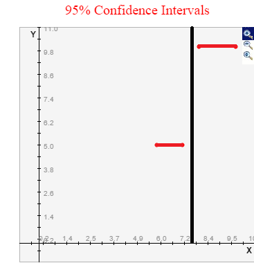 

Discussion

Conclusions

We can reject our hypothesis and say that selecting for longer leaf lengths in the P Generation did not result in a longer leaf average in the F1 Generation. Evidence for this is that the mean of the F1 Generation is less than the mean of the P Generation. This means that the average leaf length for the F1 Generation is less than the Parent Generation’s average leaf length.  Also, the CI of the F1 Generation is a lower range of values than the P Generation. The parameters of the F1 population is between 5.83 mm and 7.09 mm and for the P Generation, it is between 7.94 mm and 9.74 mm. This shows that the true value of the F1 Generation is less than the true value of the P Generation, or that the F1 Generation is expected (with a 95% degree of certainty) to have a leaf length that is smaller than that of the Parent Generation. We can also conclude that there is a possibility that leaf length is not a genetic trait. If it is not a genetic trait and the leaf lengths occur at random, it would make sense that any selection pressure we would use would not work. In order to definitely conclude this, I believe that at least 2 more trials need to be conducted. These results are surprising. I did not expect to see the average leaf length of the plants to decrease instead of increase. I was under the assumption that leaf length was a genetic trait, however, I know now that it might not be the case.

Experimental Evaluation

I was uncertain with how the initial procedure would work because at the beginning, we all seemed pretty unsure of what to do. However, as the experiment progressed, I believed we gained a better understand of what we needed to do and what we should get out of this, especially since we were learning about evolution (more specifically artificial selection) during this time. Because of this, I feel pretty confident in how we conducted the experiment. Even though I feel confident in how we conducted the experiment, I still think there may have been some spots where human error may have skewed the results. We may have agreed on what constituted as the length of the leaf, but there may have been some misreadings of the leaf length measurements. We protected ourselves against human error in terms of calculating the mean, median, standard deviation, etc because we did it using Excel and the functions within the program.

In terms of limitations, I believe the fact that not all of the seeds in the P Generation grew for the selection process is one. Another one would be that not all the seeds in F1 Generation grew. The 21 seeds that did not grow may have been sides that had leaf lengths 12 mm and above which would change the outcome of the experiment. 

In terms of the results, I believe that we need to do at least two more trials to ensure of the validity of our results. I tried researching if there was any published material on the premise of our experiment, but there was nothing I could see. Because of that, there is no real way of knowing if leaf length is a genetic trait unless we do more trials.  

References

*Confidence Interval “definition” was adapted from the McGraw Hill Criminal Justice Book*

Link: http://www.mhhe.com/socscience/crimjustice/stat-methods/book1/chap9.mhtml

Jazmean's Cell Size and Diffusion Argumentation

Cell Size and Diffusion Argumentation

Diffusion is the random motion of atoms or molecules from an area of high concentration to an area of low concentration. Diffusion is a mode of passive transport for cells because no energy is required for it to happen. Cells use diffusion in order to move atoms or molecules in and out of the cell. Through this process, a cell can expel waste or gain vital nutrients and at the same time, grow or shrink in size. Despite this, cells are never bigger than a grain a salt (which is 0.5 mm), but can be as small as 6.5 nano meters (which is the size of hemoglobin). So this begs the question, "Why are cells so small?". This is what my group members and I investigated in class. We were presented with two explanations as to why cells are small.  Explanation 1 stated that cells that have a larger surface area to volume ratio are more efficient at diffusion essential nutrients. Explanation 2 stated that the rate of diffusion is related to cell size and that nutrients diffuse at a faster rate through small cells than they do through large cells. Due to the data that was collected, there is no clear explanation that is the most valid or acceptable. 

Our group had the follow materials available for us to use: Agar (a green/blue gelatinous substance that is obtained from algae), weak acid (vinegar), beakers, a stopwatch, rulers, and plastic knives. The agar was in a container. We took the agar from the container and cut the agar into cube-like shapes (in reality they are rectangular prisms).  

Displayed are the measurements of the cubes: 

Cubes (Before Diffusion) (Outer Cube)	Length	Width	Height
1 (Small)	2 cm	2 cm	1.5 cm
2 (Big)	3.5 cm	3.5 cm	1.7 cm
3 (Big)	3.5 cm	3.5 cm	1.6 cm
4 (Small)	1.9 cm	1.9 cm	1.5 cm

We then placed the cubes into a container filled with vinegar at the same time. When the cubes hit the vinegar, the stopwatch started to keep time. At 7.3 seconds, the color started to change. Due to time restrictions, we were not able to have our cubes be fully diffused. At 32 minutes and 9 seconds, we stopped the experiment and pulled the cubes out.

Because of the time restrictions and our cubes not being fully diffused, we had to take measurements of the cube not diffused yet. 

Not Diffused Cube Measurements (inner cube)	Length	Width	Height
1 (Small)	1 cm	0.8 cm	0.7 cm
2 (Big)	2.5 cm	2.5 cm	0.5 cm
3 (Big)	2 cm	2.5 cm	0.9 cm
4 (Small)	0.9 cm	0.5 cm	0.5 cm

We then had to calculate the diffusion rates. We had to calculate the distance of the length, width, and height out each outer and inner cube by subtraction the big length from the small length and dividing that number by
two. 

Explanation given to my group by Mr. Hammer

How to Calculate Cube Diffusion Rates (Repeat for all Cubes)

side one= big length - small length/ 2

side two= big width - small width/ 2

side three= big height - small height/ 2  

Displayed below is the results.

Cubes	Length	Width	Height
1	0.5	0.6	0.4
2	0.5	0.5	0.6
3	0.75	0.5	0.35
4	0.5	0.7	0.5

We then averaged the length, width, and height in order to make the process easier. And to find the rate, we took the averages and divided it by the time the cubes stayed in the vinegar. The time was changed from minutes into seconds. So instead of it being 32.9 minutes, the time was changed to 1,929 seconds. 

Averaged Diffusion Rates

	Rate of Diffusion
Cube 1	.000259 cm/sec.
Cube 2	.000276 cm/sec.
Cube 3	.000276 cm/sec.
Cube 4	.000294 cm/sec.

In addition to calculating the rates of diffusion of each cube, we also calculated the surface area and volume of each cube. If you compile all the data into one chart, this is what it looks like:

Cubes	Volume	Surface Area	Ratio (SA to V)	Rate of Diffusion
1 (small)	6	20	10 : 3 (3.33)	.000259 cm/sec
2 (big)	20.825	48.3	48.3 : 20.825  (2.32)	.000276 cm/sec
3 (big)	19.6	46.9	46.9 : 19.6   (2.39)	.000276 cm/sec
4 (small)	5.415	18.6	18.6 : 5.415   (3.43)	.000294 cm/sec

As you can see by our final data table, we have conflicting data. For Explanation 1 to be the most valid, the cubes with a larger surface area to volume ratio should have a faster rate of diffusion. This would be true if Cube 1 was not apart of the data table. Cube 1 has a surface area to volume ratio of 10 : 3 and has a rate of diffusion of .000259 cm/sec. However, Cube 2 and 3 have a ratio of 48.3 to 20.825 and 46.9 to 19.6 (respectively) and a rate of diffusion of .000276 cm/sec. Cube 2 and 3's ratios are smaller than Cube 1's but their rate of diffusion is faster than that of Cube 1's. This means that Cube 2 and 3 would be more efficient in diffusion nutrients to the center of the cell than Cube 1. Despite this, Cube 2 and 3 have a smaller surface area to volume ratio and a slower rate of diffusion compared to Cube 4. Cube 2, 3, and 4 support Explanation 1. 

For Explanation 2 to be the most valid, the smaller cubes would have a faster diffusion rate compared to the larger cubes. Cube 4 is the one of the small cubes and it does have a faster diffusion rate compared to the larger cubes. However, Cube 1 is also one of the small cubes but it does not have a faster diffusion rate compared to the larger cubes. 

If you were to ignore Cube 1, Explanation 2 would be the most valid explanation. Cube 3 has a larger surface area to volume ratio, but has the same rate of diffusion has Cube 2. This would disprove Explanation 1. However, because the difference between the ratio is not drastic, one could infer that the small difference would not effect the rate of diffusion drastically either. Because of the conflicting data, I would not feel right as a scientist to call for one side. Further trials need to be conducted in order to solidify the data in order to pinpoint which Explanation is the most acceptable. 

Further Thoughts

These explanations can go hand in hand if you think about it. If you increase the surface area to volume ratio of a cube for example, the size of the cube gets decreases. This is the same for a cell. If you increase the SA to V ratio of a cell, its size decreases. A large SA to V ratio limits how big a cell can get. If a large SA to V ratio makes diffusion more efficient for a cell, it might make sense as to why people think smaller cells diffuse faster than larger cells; it's because their surface area to volume ratio is large.