Jazmean's Wisconsin Fast Plants Mini Lab

Jazmean Williams

The Effect of Selection Pressures on the Average Leaf Length of Wisconsin Fast Plants

Research Question and Hypothesis

Research Question: Does selection for average leaf length in the Parent Generation influence F1 phenotypes?

Hypothesis: Selection for longer leaf lengths in the P Generation results in a longer leaf average in the F1 Generation due to directional selection.

Results

P Generation Pre-Selection

After planting the seeds and giving them time to grow, the class observed the plants on Day 5 of the experiment. Discussion ensued after looking at the plants and we decid selection process. We then gathered data from the plants. For the P Generation before selection, there were 57 plants. Each student in the class measured the leaf lengths of each plant quad (Figure 1). The measurements of the average leaf lengths of each separate plant aided in deciding which plants were able to stay in the experiment and which ones were cut. After finding what the average leaf lengths were, we graphed the data in the form of a histogram (Figure 2). This was done to see if there was a variation of leaf lengths in this generation and if leaf length was a trait that could be used in the selection process. The histogram showed that there was a variation of leaf lengths in the P Generation and that leaf length could be used in the selection process. The class determined that we were going to selected against small leaf lengths and we chose 12mm as our cut off length. This means that if at least one of the leaves of the plants were 12mm or more, they stayed. If the plant contained no leaves that were at least 12mm, they were cut. The average leaf length of each plant also helped in determining the median and mean leaf length of the P Generation which was 8.5mm and was 8.839mm respectively. We also found the Standard Deviation, SEM, and Confidence Intervals of this generation. Figure 3 shows all of the data collected from the P Generation before selection.

Figure 1



Figure 2

                     

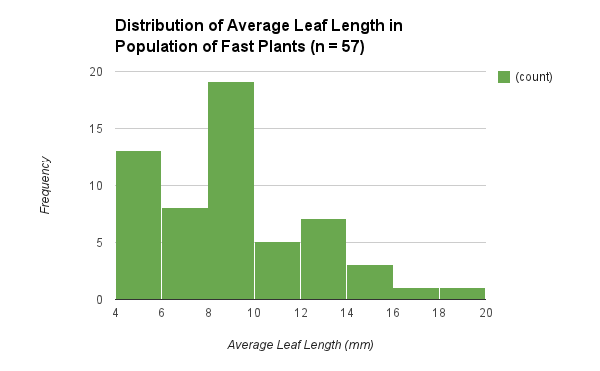
Figure 3

	P Generation
Sample Size (n)	57
Mean	8.839181287 mm
Median	8.5 mm
Standard deviation	3.39196426 mm
SEM	0.4492766416 mm
95% CI Lower Limit	7.940628004 mm
95% CI Upper Limit	9.73773457 mm

P Generation After Selection

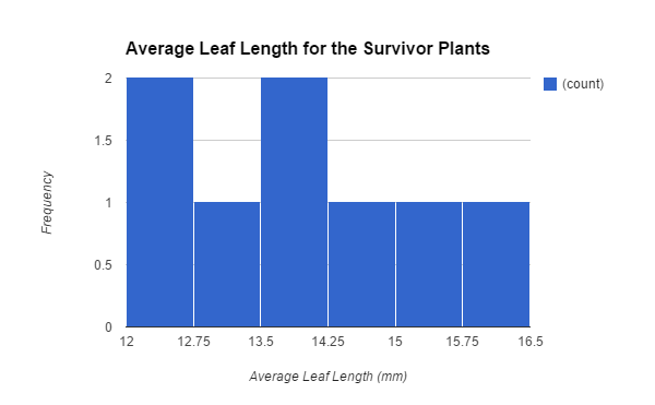
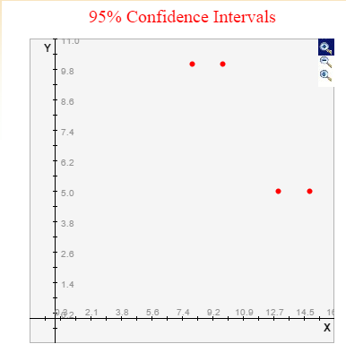
After the P Generation underwent the selection process, only 8 plants remained. We calculated the mean and median of the survivor generation which were 13.88 mm and 13.75 mm respectively (Figure 4).  We also calculated the average leaf lengths of the plants and made a histogram of the data (Figure 5). The histogram provided us with a visual representation to see if the leaf lengths were 12mm and above and we selected correctly. To reaffirm that we really did the selection process correctly, we found the Standard Deviation and SEM which helped us find the Upper and Lower Confidence Intervals of the P Generation Survivors. We then compared the intervals with the P Generation Confidence Intervals. Confidence Intervals gives us the parameters of a population. They provide a range of values that, with a certain degree of confidence (in this case, 95%), tell us where the “true” population values fall. If the Confidence Intervals of the P Generation and the P Generation Survivors overlap, we know that they both have a chance of having a plant with the same leaf length. We do not want this since we are selecting against leaf lengths shorter than 12mm. The overlap between the two intervals would also tell us that we did our selection process wrong. Luckily, the two confidence intervals did not overlap (Figure 6). Knowing this allowed us to continue with our experiment. We cross pollinated the plants on Days 12 to 16 of the experiment. After drying the seed pods, we counted 54 seeds in total and replanted them.

Figure 4

	P Generation - Survivors
Sample Size (n)	8
Mean	13.88 mm
Median	13.75 mm
Standard deviation	1.26 mm
SEM	0.45 mm
95% CI Lower Limit	12.98 mm
95% CI Upper Limit	14.78 mm

Figure 5

Figure 6

(Top dots are P Generation and bottom dots are P Generation Survivors)

F1 Generation

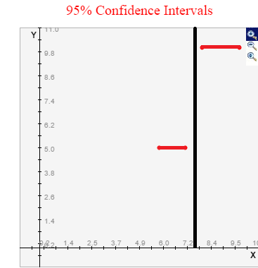
Out of the 54 seeds that were planted, only 33 sprouted and grew into plants. We then measured the leaf lengths of each plant and took the average. After that, we calculated the mean and the median. Right away we saw that the mean and the median of the F1 Generation was lower than that of the P Generation (Pre-Selection). The mean and the median of the F1 Generation were 6.46 mm and 6.33 mm respectively (Figure 7), while the mean and median of the Parent Generation were 8.839 mm and 8.5 mm respectively. With this in mind, we continued and made a histogram of the average leaf length of the F1 Generation to visually see the distribution of the leaf lengths (Figure 8). The histogram shows that the majority of the plants had an average leaf length between 6mm and 7.5mm which lines up with the values we found for the mean and median. We then found the Standard Deviation, SEM, and Confidence Intervals. We compared the confidence intervals of the F1 Generation and Parent Generation to see if there was any overlap. Figure 9 shows that there was no overlap between the two generations. Because there was no overlap, with a 95% degree of certainty, we can say that the F1 Generation and P Generation do not have the same leaf length values.

Figure 7

	F1 Generation
Sample Size (n)	33
Mean	6.462121212
Median	6.333333333
Standard deviation	1.80735
SEM	0.3146201419
95% CI Lower Limit	5.832880928
95% CI Upper Limit	7.091361496

Figure 8

The top line is the P Gen and the bottom line is the F1 Gen. The black line between the two red lines helps distinguish the gap between the two intervals. 

Discussion

Conclusions

We can reject our hypothesis and say that selecting for longer leaf lengths in the P Generation did not result in a longer leaf average in the F1 Generation. Evidence for this is that the mean of the F1 Generation is less than the mean of the P Generation. This means that the average leaf length for the F1 Generation is less than the Parent Generation’s average leaf length.  Also, the CI of the F1 Generation is a lower range of values than the P Generation. The parameters of the F1 population is between 5.83 mm and 7.09 mm and for the P Generation, it is between 7.94 mm and 9.74 mm. This shows that the true value of the F1 Generation is less than the true value of the P Generation, or that the F1 Generation is expected (with a 95% degree of certainty) to have a leaf length that is smaller than that of the Parent Generation. We can also conclude that there is a possibility that leaf length is not a genetic trait. If it is not a genetic trait and the leaf lengths occur at random, it would make sense that any selection pressure we would use would not work. In order to definitely conclude this, I believe that at least 2 more trials need to be conducted. These results are surprising. I did not expect to see the average leaf length of the plants to decrease instead of increase. I was under the assumption that leaf length was a genetic trait, however, I know now that it might not be the case.

Experimental Evaluation

I was uncertain with how the initial procedure would work because at the beginning, we all seemed pretty unsure of what to do. However, as the experiment progressed, I believed we gained a better understand of what we needed to do and what we should get out of this, especially since we were learning about evolution (more specifically artificial selection) during this time. Because of this, I feel pretty confident in how we conducted the experiment. Even though I feel confident in how we conducted the experiment, I still think there may have been some spots where human error may have skewed the results. We may have agreed on what constituted as the length of the leaf, but there may have been some misreadings of the leaf length measurements. We protected ourselves against human error in terms of calculating the mean, median, standard deviation, etc because we did it using Excel and the functions within the program.

In terms of limitations, I believe the fact that not all of the seeds in the P Generation grew for the selection process is one. Another one would be that not all the seeds in F1 Generation grew. The 21 seeds that did not grow may have been sides that had leaf lengths 12 mm and above which would change the outcome of the experiment. 

In terms of the results, I believe that we need to do at least two more trials to ensure of the validity of our results. I tried researching if there was any published material on the premise of our experiment, but there was nothing I could see. Because of that, there is no real way of knowing if leaf length is a genetic trait unless we do more trials.  

References

*Confidence Interval “definition” was adapted from the McGraw Hill Criminal Justice Book*

Link: http://www.mhhe.com/socscience/crimjustice/stat-methods/book1/chap9.mhtml

Nida Ali's Fast Plant Mini Lab

Nida Ali

Analysis

In this class collaborative lab, we examined the effect on the average leaf length   plays on Wisconsin Fast Plants based off of artificial selection.

Primarily, a histogram was constructed to display the leaf length of our first generation plants. However majority of the leaf lengths were similar to one another, which thus did not formulate a bell curve graph for the parent population before selection (Figure 1). Then the artificial selection part of the lab began when we began to select for traits that are able to display a bell curve based on collected data. We then collected the average leaf length of each individual plant and constructed the histogram below. As depicted, this histogram clearly displays a bell curve based off the average leaf length per plant rather than each individual leaf length on a plant. On average the mean of the parent population was 8.8mm and the median was 8.5mm. Most of the leaf lengths of the plants fall in 4mm-10mm mark and the outliers fall after the 14mm mark. The histogram below displays a bell curve mainly because of the 95% Confidence Intervals that is 7.94 to 9.74, the standard deviation of 3.39 and SEM of .45.

Figure 1

After day 9, we began to look for variation among the plants. We selected for plants with the longest leaf length of 12mm long as our variable trait since it varies within range and kept those leaves alive, which ended up being just 8 plants. Leaves the were under 12mm were cut off and no longer remained in this artificial plant selection lab. As shown in the histogram below of the parent population after selection (Figure 2), the average leaf length of plants dramatically altered through augmentation. The parent population after selection histogram below does not present a bell curve, unlike the histogram of P generation before selection (Figure 1), which thus states that the average leaf lengths were similar in height. Majority of the plants had an average leaf length between 12mm to 14.25mm. As for the mean, the average increased from 8.8mm, before selection from the parent population,  to 13.88mm after selection. Likewise, the median also increased from before and after selection of the parent population from 8.5mm to 13.75mm. The standard deviation had a minor decrease from the P generation before survivors from 3.39 to 1.26, which thus displays that among the plants, not much change/variation was depicted. 

Once the parent population survivors reproduced, the difference seen among the mean and 95% confidence intervals were much closer to the parent population before selection rather than the parent population after selection. We calculated 95% intervals in order to see if the artificial selection process was done correctly. If the 95% intervals overlapped, the average leaf lengths were similar. In contrast, if the 95% intervals did not overlap, the average leaf length were not similar. The 95% confidence intervals were not similar either which highlights that the two do not overlap. In addition, the SEM value of 4.449 remained relatively the same to that of the P generation before survivors.

Figure 2

A proper bell curve graph was seen after my classmates and I took measured the average leaf lengths for each plant that was pollinated with beesticks. During this process, only a few plants survived, in which we based the histogram below off of. The F1 generation histogram (Figure 4)  displays a better bell curve more than but similar to that of the parent generation before selection. The medium of the average leaf lengths is 6.3mm and the mean averaged out to 6.5mm. The SEM was of 0.31 and the standard deviation was 1.81. The selection for the parent generation before selection influences the F1 generation due to the similar values seen in the means, 95% lower limit and upper limit. While comparing the 95% confidence intervals of the upper and lower limit of the parent generation of 7.9 to 9.73 to that of the F1 generation of 5.8 to 7.09, they do not overlap resulting in less similarity.

Figure 4

Discussion

Conclusion:

The null hypothesis that there is no significant difference is seen between the two means of the parent generation before selection and F1 generation is rejected. We reject the null hypothesis because there is a significant difference among the means due to the difference seen in the P generation before selection and F1 generation 95% confidence intervals. The 95% confidence intervals do not overlap, which thus states that they were not similar. Since the leaf length means of the P generation Survivors and Offspring generation are not similar, the artificial selection for the average leaf length does not influence the offspring generations. Through this experiment, I can conclude that the role artificial selection does not largely impact generations since the trait that is selected against may in fact be randomly passed down through generations.

A few limitations occurred during this lab experiment. One limitation is that not all of the planted seeds were able to grow, which thus resulted in several plants dying out and not participating in the experiment. Therefore, our results ended up being based off of 8 plants total. In addition, another limitation is that we did not regularly monitor our plants due to the lack of time, in most cases. We only monitored the plants once the next step in the lab was about to be conducted. Therefore, if we were consistent in monitoring our plants, possibly more plants would have been produced and not dried out due to any shortages either to light or water. If more plants were produced during this lab, accurate results would have been seen.

Experimental Evaluation:

Several errors conducted during this experiment may have altered the end result of this lab if they were addressed earlier. First and foremost, a huge error that was conducted was not exactly keeping track of the days. If we focused on what needs to be done mandatory on certain days, then I believe we would have accurate results. By going a few days here and there may not, at first, seem like a massive implication, but it may massively alter our results by allowing the plants to grow a couple of more days. One common error is not properly averaging the leaf lengths. In most cases, this may have to do with the shortage of time which resulted in students to quickly rush their math conducting process. In addition, another error that may alter the end result of the experiment would be accurately trimming the plants that were no longer needed in this lab.

Even though this lab was very time consuming, considering the few months that it took to fully conduct this lab, I felt that the results we received were still sufficient to an extent regarding minor errors.

Sara's Fast Plant Mini Lab Report

The Effects of Artificial Selection on Fast Plants

Calculations & Statistical Analysis:

Figure 1:

For this experiment we measured all of the individual leaf lengths for each plant and calculated the average leaf length for each plant. A histogram of the average leaf length of all the plants  was created with a sample size of 57(figure 1).  The graph is not a bell curve shape but, instead is skewed.  The histogram shows that most of the plants have an average leaf length from 4mm to 10mm. The histogram also shows that there were a few plants that had extremely high leaf lengths of 18mm and 20mm. With the average leave lengths mostly being below 10 mm caused for the skew shape of the graph (Figure 1).  The average  length of the parent population is 8.84 mm and the median is 8.5 mm. The SEM was about .45 and a standard deviation of about 3.39 which, would have caused the the histogram to appear skewed.   The 95% CI is 7.94 to 9.74 which, would have contributed to the histogram to be skewed due to the spread of the data(Figure 1). 



Figure 2: 
  As a class we decided to select for plants with an average leaf length of 12 mm or higher therefore, we cut the plants who did not fit that criteria. We ended up with 8 plants as survivors after the selection (shown in Figure 2). The graph is not a bell curve just like the graph of the population before the selection (Figure 1 and 2).  The shape changed due to the change in the data. The mean of the data is 13.88mm and the median is 13.75mm which, would have caused the graph to shift.  The standard deviation is 1.26 which, shows that there was not much of a fluctuation in the data in Figure 2. However, the P generation had a higher standard deviation which, shows that there was more spread of data (as shown in Figure 1). The SEM was 0.45 and there was a 95% CI of 12.98 to 14.78.  This 95% CI of the survivors was not significantly than the 95% CI of the P generation since the two do not overlap each other (Figures 1and 2).

Figure 3: 
The last set of data collected was the average leaf length for all of the plants in the next generation.  This data was collected on Day 9 after planting of the first generation of offspring of the survivors. We did the same thing we did the other two times we had collected data which, was measure all the leaves per plant and then average the length of those leaves.  Then those values were graphed in a histogram.   This histogram is more of a bell curve shape but, slightly more to the left side.That would be because there were more plants with average leaf lengths that were lower. The mean of the average leaf lengths is about 6.5mm and the median of the the data is 6.3mm (Figure 3).  The histogram shows that most of the plants had an average leaf length from 6 mm to 7.5 mm ( Figure 3). There were only few that had an average leaf length from 10.5 mm to 12mm.  There was a standard deviation of about 1.81 with a SEM of about 0.31.  Compared to the survivors (Figure 2) the standard deviation for the F1 generation is higher which shows that there was more of a spread of data because there are more plants that were planted.  The 95% CI is 5.83 to 7.09 and it doesn’t overlap the 95% CI of the survivors (Figure 2) which, means that they are not significantly close to each other.  The F1 95% CI does overlap the P generation (Figure 1) a little which, means that they are significantly close to each other.







   Discussion:
Conclusion:
The experiment conducted relates to the evolution domain in the course and specifically with artificial selection.  By doing this lab I was able to see that artificial selection sometimes doesn’t always mean that the trait selected for is not necessarily a gene that is passed down from generation to generation rather it is a random trait. That is based off the evidence shown in the F1 generation (figure 3) with the mean being lower than the survivors after the selection (figure 2).  Also with the 95% CI not overlapping it showed that they were not significantly close.  If the trait was able to be passed down the two 95% CI should overlap due to the fact that the points in the F1 generation would be higher since the average leaf length would be higher. Also that the lengths would be similar to those of their parents since that is where the trait came from.  As shown in Figure 3 the average leaf lengths of the plants are mainly low and few are 12mm or higher unlike the average leaf lengths in Figure 2.   Therefore, based on that data the results did not turn out the way I had hypothesized.   Some limitations in the experiment could have lead to the results to be different from expected.  One limitation would be keeping the plants 10 cm from the light that was provided.  We used textbooks to regulate the distance but, once the plants grew and one textbook was removed it was hard to keep the plants at the right distance.  Reason being that by removing the last textbook would make the plants too far away from the light and the textbook kept the plants a little too close as well.

Experimental Evaluation: 
However, errors could have altered the outcome of the experiment.  For instance, we might not have measured the plants on the wrong day from what the experiment called for.  This could be due to there not being enough time in class to do so or forgetting or the 9th day which the leaves were suppose to be measured fell on a weekend.  That would lead to the leaves being able to grow a little longer which, made the averages bigger.   Another error would be the measurements of the leaves could be off and the math done for the averages could have been wrong as well which, would have lead to altered data.  Therefore, leads to different results.  Lastly, when cutting the plants that didn’t have an average leaf length of 12mm or higher could have been a source of error because too many could have been cut which, leads to a different amount of survivors.  The fact that no one had recorded the number of survivors is an error because when doing final calculations knowing the exact number of survivors would have lead to more accurate results.  If this experiment was done over then the math would have been done twice to ensure accuracy and the measuring could be done by two people as well for the same reason.  The cutting of the plants would have also be done more carefully by making sure that the right ones are being cut by double checking the data collected. Then recording the number of the survivors in order to have the correct amount in order to have more accurate calculations in the end.  Lastly, in regards on keeping track on what day of the experiment we were on would be done better in order to make measurements and steps are done at the right time in order to make sure that more accurate data could be collected.